
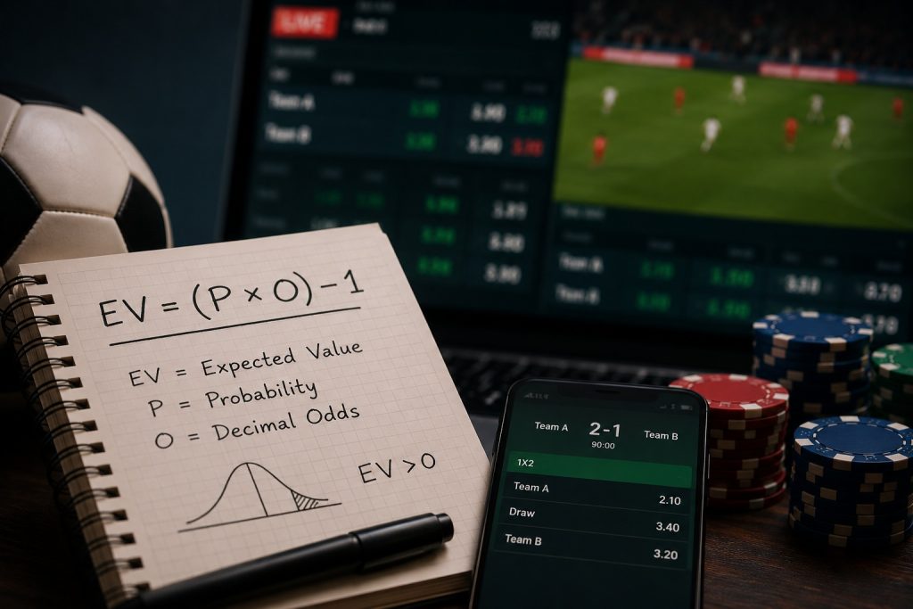
Expected value is one of the most important concepts in sports betting, yet it is also one of the easiest to misunderstand.
A bet can win and still be a bad bet. A bet can lose and still have been the correct decision. That sounds strange at first, especially if you are used to judging a betting strategy by the number of winning tickets, but expected value looks at something different: the relationship between the probability of an outcome and the price being offered for it.
If you believe a team has a 55% chance of winning and a sportsbook is offering odds that imply only a 50% chance, there may be value in that price. If the same team is offered at a price implying a 65% probability, the bet may be a poor one even though you still believe the team is more likely than not to win.
That distinction is the foundation of value betting.
Expected value, usually shortened to EV, gives you a mathematical way to measure that difference. In its simplest form, it answers a straightforward question:
If I could place this exact same bet over and over again at the same odds and with the same underlying probability, how much would I expect to win or lose per bet?
The calculation itself is relatively simple.
The difficult part is estimating the probability accurately.
This guide explains how to calculate expected value in sports betting from the ground up, how to convert odds into implied probability, how bookmaker margins affect the calculation, how to remove the margin from a market, and how to recognise whether a supposed +EV bet is actually based on a reliable probability estimate.
The basic idea behind expected value
Expected value comes from probability theory.
In betting, every possible outcome has a probability and a financial result attached to it. EV combines those two things into one number.
For a simple two-outcome bet, you have:
- a probability of winning
- a probability of losing
- a profit if the bet wins
- a loss if the bet loses
The general formula is:
EV = (Probability of winning × Profit if you win) − (Probability of losing × Amount lost)
For a $100 bet, imagine you believe a team has a 55% chance of winning and the sportsbook offers decimal odds of 2.00.
At 2.00, a $100 winning bet produces $100 in profit.
The calculation is:
EV = (0.55 × $100) − (0.45 × $100)
EV = $55 − $45
EV = +$10
That means the expected profit is $10 per $100 staked.
It does not mean you are guaranteed to make $10.
The team can lose the next match and you lose your entire $100 stake.
EV describes the mathematical average over a large number of repetitions, not the result of one individual bet. This distinction is central to understanding value betting.
The easiest EV formula for decimal odds
For bettors using decimal odds, the calculation can be simplified considerably.
The formula is:
EV = (True Probability × Decimal Odds) − 1
If you want the result as a percentage:
EV% = [(True Probability × Decimal Odds) − 1] × 100
Suppose you estimate that Arsenal have a 45% chance of winning a particular match and a bookmaker offers odds of 2.40.
The calculation is:
EV = (0.45 × 2.40) − 1
EV = 1.08 − 1
EV = +0.08
Therefore:
EV = +8%
In theoretical terms, you would expect to make $8 for every $100 wagered if you could repeatedly place the same bet at 2.40 with a genuine 45% probability.
This simplified formula is mathematically equivalent to the longer probability-weighted profit calculation.
Why the probability estimate matters more than the formula
This is where most discussions about expected value become too simplistic.
The formula is easy.
Your probability estimate is the difficult part.
Anyone can type:
0.55 × 2.10 − 1 = +15.5%
The real question is:
Why do you believe the probability is 55%?
If that 55% is simply a feeling because “Team A has been playing well”, the +15.5% EV figure is not particularly meaningful.
You have not discovered a 15.5% edge.
You have simply entered an uncertain assumption into a calculator.
A serious EV process therefore has two separate stages:
Stage 1: Estimate the probability.
Stage 2: Compare that probability with the available price.
The second stage is easy.
The first stage is where the actual analytical work happens.
A recent academic study examining football and tennis betting markets also highlights the limitations of treating raw inverse odds as perfect estimates of outcome probabilities, particularly because bookmaker margins and market structure need to be accounted for.
How to convert betting odds into implied probability
Before calculating EV, you should understand what the bookmaker’s odds are saying.
With decimal odds, the formula is extremely simple:
Implied Probability = 1 ÷ Decimal Odds
Here are some common examples:
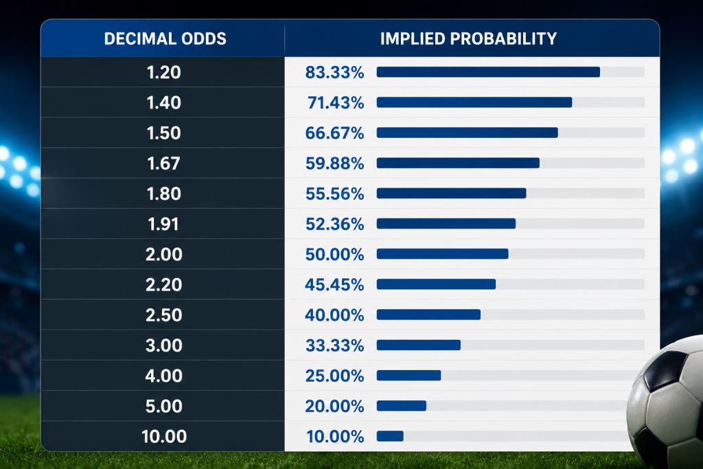
So if a bookmaker offers 2.50, the price implies a 40% probability.
If your estimated true probability is 45%, you potentially have an edge.
If your estimate is 35%, you do not.
That is the basic relationship behind value betting.
The break-even probability
One of the most useful ways to look at odds is through the break-even probability.
The break-even probability is the win rate you need to achieve in order to avoid losing money at a particular price, ignoring other factors.
For decimal odds:
Break-even Probability = 1 ÷ Decimal Odds
So:
1.50 → 66.67%
2.00 → 50%
2.50 → 40%
3.00 → 33.33%
5.00 → 20%
This immediately gives you a framework for evaluating a bet.
Suppose you believe a team has a 42% chance of winning.
At odds of 2.20, the break-even probability is:
1 ÷ 2.20 = 45.45%
Your probability estimate is only 42%.
That is a negative-EV bet.
Now imagine another sportsbook offers 2.50.
The break-even probability becomes:
1 ÷ 2.50 = 40%
Your estimate of 42% is now higher than the market’s break-even probability.
The same team, the same match and the same opinion have suddenly become a potential value bet.
The price changed.
That is one of the most important lessons in sports betting.
Your opinion does not create value by itself.
The difference between your probability and the available price creates the value.
A complete expected value example
Let’s use a football match.
Suppose Manchester United are playing Liverpool.
You analyse the fixture and estimate:
Manchester United win probability = 48%
A sportsbook offers:
Manchester United = 2.30
First, calculate the implied probability:
1 ÷ 2.30 = 43.48%
The bookmaker’s price therefore requires a win probability of approximately 43.48% to break even.
Your model says 48%.
Now calculate EV:
EV = (0.48 × 2.30) − 1
EV = 1.104 − 1
EV = +0.104
So:
EV = +10.4%
For every $100 staked, the theoretical expected profit is $10.40 if the assumptions remain valid over a very large number of identical bets.
That is a substantial theoretical edge.
But there is an important warning.
A 48% probability estimate must be credible.
If the real probability is actually 42%, the entire calculation changes:
0.42 × 2.30 − 1 = −3.4%
The apparent +10.4% edge disappears and becomes negative.
This is why EV betting is fundamentally a probability-estimation problem.
What is a +EV bet?
A +EV bet is a bet with positive expected value.
In decimal odds:
+EV when:
True Probability × Decimal Odds > 1
Or, equivalently:
True Probability > 1 ÷ Decimal Odds
For example:
You estimate the probability at 55%.
The odds are 2.00.
0.55 × 2.00 = 1.10
Therefore:
EV = +10%
That is a +EV bet.
A -EV bet works the opposite way.
Suppose your probability estimate is 55%, but the bookmaker offers 1.70:
0.55 × 1.70 = 0.935
EV = −6.5%
You can still win the bet.
But the price is not attractive relative to your estimated probability.
What is a -EV bet?
A negative-EV bet has an expected loss over repeated trials.
Suppose your estimated probability is 40%.
The sportsbook offers 2.20.
The break-even probability is:
45.45%
Your estimate is below the break-even level.
EV:
0.40 × 2.20 − 1 = −0.12
So:
EV = −12%
If your probability estimate is correct, you would expect to lose $12 per $100 wagered over a very large sample at that exact price.
This does not mean the next bet will lose.
It could win immediately.
That is precisely why individual results are a poor way of judging whether a betting decision was good.
Why a winning bet can be a bad bet
Imagine you bet $100 on a team at 1.80.
You estimate that the team has only a 50% chance of winning.
The implied probability at 1.80 is:
55.56%
Your probability is lower.
Therefore:
EV = 0.50 × 1.80 − 1
EV = −10%
The team wins.
You collect $80 profit.
Was it a good bet?
Mathematically, no.
You made a profitable result on a negative-EV decision.
This distinction is incredibly important.
The result of the bet and the quality of the bet are two different things.
Over a single game, luck dominates.
Over a sufficiently large number of bets, the underlying expected value becomes increasingly important.
Why a losing bet can be a good bet
Now reverse the situation.
You estimate a team has a 55% chance of winning.
The sportsbook offers 2.10.
The implied probability is:
1 ÷ 2.10 = 47.62%
Your EV is:
0.55 × 2.10 − 1 = +15.5%
You place the bet.
The team loses.
Was it a bad bet?
No.
If your 55% probability estimate was accurate and the price really was 2.10, the decision was positive EV.
The outcome simply went against you.
This is the psychological side of value betting that many bettors struggle with.
A good process can produce losing bets.
A bad process can produce winning bets.
The objective is not to win every bet.
The objective is to consistently make decisions where the price is better than the probability warrants.
The bookmaker margin changes everything
There is one major complication.
Sportsbooks do not normally offer fair odds.
They build a margin into their markets.
This is known as:
- bookmaker margin
- overround
- vig
- juice
In a perfectly fair two-way market, the probabilities would add up to 100%.
For example:
Team A = 50%
Team B = 50%
Fair decimal odds would be:
2.00 / 2.00
But a sportsbook might offer:
1.91 / 1.91
Each price implies:
1 ÷ 1.91 = 52.36%
Combined:
52.36% + 52.36% = 104.72%
The market percentage is therefore 104.72%.
The overround is:
104.72% − 100% = 4.72%
This is the built-in margin.
Academic and industry analyses use this same inverse-odds approach to calculate the overround and infer underlying probabilities from quoted prices.
How to calculate bookmaker margin
For decimal odds, the formula is:
Overround = Σ(1 ÷ Odds) − 1
For a two-way market:
Overround = (1 ÷ Odds A) + (1 ÷ Odds B) − 1
For a football 1X2 market:
Overround = (1 ÷ Home Odds) + (1 ÷ Draw Odds) + (1 ÷ Away Odds) − 1
Imagine:
Home = 2.00
Draw = 3.40
Away = 4.00
Calculate the probabilities:
Home:
1 ÷ 2.00 = 50%
Draw:
1 ÷ 3.40 = 29.41%
Away:
1 ÷ 4.00 = 25%
Total:
50% + 29.41% + 25% = 104.41%
Therefore the overround is:
4.41%
That 4.41% is why simply treating the raw implied probabilities as true probabilities can be misleading.
How to remove the bookmaker margin
If you want to estimate a market’s no-vig probabilities, you can normalise the implied probabilities.
Take the previous example:
| Outcome | Odds | Raw implied probability |
|---|---|---|
| Home | 2.00 | 50.00% |
| Draw | 3.40 | 29.41% |
| Away | 4.00 | 25.00% |
| Total | 104.41% |
To remove the overround, divide each raw implied probability by the total market probability.
For the home team:
50 ÷ 104.41 = 47.89%
For the draw:
29.41 ÷ 104.41 = 28.17%
For the away team:
25 ÷ 104.41 = 23.94%
Now the probabilities add up to approximately 100%.
These are often called no-vig, fair or normalised probabilities.
They are not guaranteed to be the true probabilities.
They are simply a way of removing the bookmaker’s built-in overround from the quoted market.
Why comparing sportsbooks is so important
Suppose one sportsbook offers:
Team A = 2.00
Another offers:
Team A = 2.10
Your probability estimate does not change.
But the EV does.
At 2.00 with a 52% probability:
0.52 × 2.00 − 1 = +4%
At 2.10:
0.52 × 2.10 − 1 = +9.2%
The difference between those prices is enormous from an EV perspective.
This is why odds shopping can be more valuable than finding a supposedly perfect betting prediction.
You might have the correct opinion about a match but still place a poor bet if you accept the worst available price.
A recent betting-market study also highlights how the relationship between quoted prices and underlying probabilities is more complicated than simply treating inverse odds as perfectly calibrated probabilities.
EV in American odds
Many sports betting markets, particularly in the United States, use American odds.
There are two basic forms.
Positive American odds
For positive odds:
Implied Probability = 100 ÷ (Odds + 100)
Example:
+150
100 ÷ 250 = 40%
So +150 implies a 40% break-even probability.
Negative American odds
For negative odds:
Implied Probability = |Odds| ÷ (|Odds| + 100)
Example:
−150
150 ÷ 250 = 60%
So -150 implies a 60% break-even probability.
For EV calculations, many bettors convert American odds to decimal odds first because the decimal formula is easier to work with.
+150 becomes:
2.50 decimal
-150 becomes approximately:
1.67 decimal
Then:
EV = Probability × Decimal Odds − 1
EV with fractional odds
Fractional odds are common in the UK and Ireland.
For example:
3/1
means you win $3 profit for every $1 staked.
The decimal equivalent is:
4.00
The implied probability is:
1 ÷ 4.00 = 25%
Another example:
5/2
equals decimal odds of:
3.50
Implied probability:
1 ÷ 3.50 = 28.57%
Once you convert fractional odds into decimal odds, the EV calculation is exactly the same.
How to calculate EV for a football match
Football is particularly interesting because the most common 1X2 market has three outcomes:
- Home win
- Draw
- Away win
Suppose the bookmaker offers:
Arsenal 2.10
Draw 3.60
Chelsea 3.50
You estimate:
Arsenal = 50%
Draw = 27%
Chelsea = 23%
Let’s calculate the EV of the Arsenal bet:
EV = 0.50 × 2.10 − 1
EV = +5%
The bet is theoretically +EV.
Now calculate the draw:
EV = 0.27 × 3.60 − 1
EV = −2.8%
The draw is negative EV according to your model.
Chelsea:
EV = 0.23 × 3.50 − 1
EV = −19.5%
Only Arsenal would qualify under your estimates.
This illustrates another important point:
You do not need to predict every outcome correctly.
You are looking for discrepancies between your estimated probability and the available price.
Expected value for over/under betting
The same process works for totals.
Imagine a sportsbook offers:
Over 2.5 goals = 2.10
You estimate that the probability of three or more goals is:
52%
The bookmaker’s break-even probability is:
47.62%
Your EV:
0.52 × 2.10 − 1 = +9.2%
Therefore the bet has a theoretical expected value of +9.2%.
Again, the key is the quality of the 52% estimate.
That probability could come from a model based on:
- expected goals
- historical scoring rates
- team attacking strength
- defensive strength
- injuries
- expected line-ups
- home advantage
- rest days
- tactical matchups
- weather
- market information
The more systematic the probability model, the more meaningful the resulting EV becomes.
Expected value for player props
EV also applies to player markets.
Suppose a sportsbook offers:
Erling Haaland over 3.5 shots at 2.00
You estimate that he reaches four or more shots in:
54% of comparable situations
Then:
EV = 0.54 × 2.00 − 1
EV = +8%
The same mathematics applies to:
- player goals
- shots
- assists
- passes
- tackles
- receptions
- touchdowns
- points
- rebounds
- three-pointers
- cards
The challenge is usually not the formula.
It is constructing a realistic probability distribution for the player’s performance.
For example, a player averaging 4.2 shots per match does not automatically have a 54% probability of recording four or more shots.
Average and probability distribution are not the same thing.
Expected value in accumulator bets
Accumulators require extra care.
Suppose you have three selections, each of which you believe has a 60% chance of winning.
If the outcomes were independent, the probability of all three winning would be:
0.60 × 0.60 × 0.60 = 21.6%
If the accumulator pays decimal odds of 5.00, then:
EV = 0.216 × 5.00 − 1
EV = +8%
That looks attractive.
But there is an important problem.
The assumption of independence may not be valid.
Consider an accumulator containing:
- Team A to win
- Team A over 1.5 goals
- Team A striker to score
Those outcomes are correlated.
If Team A wins comfortably, all three selections may become more likely.
You cannot simply multiply probabilities without considering the relationship between the legs.
This becomes even more important with same-game parlays, where correlations can be substantial.
Expected value in live betting
Live betting does not change the mathematics of EV.
It changes the information available to estimate probability.
In-play models can incorporate:
- current score
- time remaining
- red cards
- possession
- shots
- expected goals
- substitutions
- injuries
- game state
- tempo
Suppose a football team is 0-0 after 70 minutes.
The bookmaker offers:
Over 1.5 goals at 2.80
You estimate the probability of at least two total goals from that point at 40%.
Then:
EV = 0.40 × 2.80 − 1
EV = +12%
The theoretical edge is +12%.
But live betting creates additional complications.
Prices can move rapidly.
Markets may suspend.
Information can reach sportsbooks faster than individual bettors.
And a probability model that works before kick-off may be poorly calibrated during live play.
Expected value does not guarantee profit
This deserves its own section because it is perhaps the most common misunderstanding.
A +EV bet can lose.
A sequence of +EV bets can lose.
A strategy with positive expected value can experience a long losing run.
Why?
Variance.
Imagine a coin that genuinely lands heads 55% of the time.
You bet on heads at fair odds corresponding to a positive expectation.
You can still lose the first five flips.
You can lose ten.
You can lose more.
The fact that the underlying probability favours you does not determine the result of a small sample.
Sports betting is exactly the same.
The objective of EV betting is not to eliminate uncertainty.
It is to make the mathematical expectation favourable.
A 2023 study on optimal sports-betting decision-making similarly frames wagering as a problem of selecting outcomes that offer positive expected profit based on an estimated probability distribution rather than simply predicting winners.
EV versus win rate
A high win rate does not automatically mean a profitable betting strategy.
Imagine two bettors.
Bettor A
Wins 70% of bets.
Average odds: 1.30.
Bettor B
Wins 45% of bets.
Average odds: 2.40.
Bettor A may look far more successful because they win seven out of every ten bets.
But the price matters.
At 1.30, a bettor needs to win approximately:
76.92%
to break even.
So a 70% win rate could still be negative EV.
At 2.40, the break-even rate is:
41.67%
A bettor winning 45% of those bets could theoretically have positive EV.
This is why the question:
“How many bets do you win?”
is incomplete.
A much better question is:
“At what prices do you win those bets?”
EV versus ROI
EV and ROI are related but not identical.
EV is the expected mathematical return based on your estimated probabilities and available odds.
ROI measures your actual return relative to the amount wagered.
For example, you might have:
100 bets
$10,000 total stakes
$10,800 returned
Your actual ROI is:
8%
But that does not prove your expected value was 8%.
Your actual results can be higher or lower than expected because of variance.
Over a large sample, if your probability estimates and prices are accurate, actual ROI should tend to move closer to the underlying expected return.
Closing line value and EV
One of the most useful ways to evaluate a betting process is to look at closing line value, commonly abbreviated as CLV.
Suppose you bet Team A at:
2.20
Several hours later, the market closes at:
2.00
You obtained a better price than the closing market.
That does not guarantee your bet won.
It does suggest that your price was better than the final market price.
If this happens consistently, it can be evidence that your betting process is identifying favourable prices.
CLV is not identical to EV, and it should not be treated as a perfect replacement for a probability model.
But it is an important performance metric because it focuses on the quality of the price you obtained rather than simply whether individual bets won.
How to find your own true probability
This is the hardest part of the process.
There are several approaches.
Historical data
You can build probability estimates using historical results.
For football, that might include:
- home and away performance
- goals scored
- goals conceded
- expected goals
- shots
- shot quality
- set pieces
- player availability
- schedule strength
The danger is relying too heavily on small samples.
A team winning five consecutive matches does not automatically mean it has a 100% probability of winning its next match.
Statistical models
More sophisticated bettors can create models using:
- Poisson distributions
- expected goals
- Elo ratings
- logistic regression
- Bayesian models
- machine learning
- player-level data
Recent academic work has examined whether relatively simple football models based on xG can identify signals in betting markets. A 2026 study using Bundesliga data found that bookmaker odds were generally better calibrated statistically, while an xG-based model still captured some signals not fully reflected in market prices.
That is a useful reminder that having a model does not automatically mean having an edge.
The model has to be calibrated.
Market-based estimates
Another approach is to use a high-quality market as a probability reference.
You can compare prices across sportsbooks and use a low-margin market to estimate fair probabilities.
The advantage is that markets aggregate enormous amounts of information.
The disadvantage is that you are effectively trying to improve on a market that already contains the information and opinions of many participants.
Common mistakes when calculating expected value
Mistake 1: Using bookmaker implied probability as your true probability
If a bookmaker offers 2.00, the implied probability is 50%.
That does not mean the true probability is exactly 50%.
The bookmaker has a margin.
You need an independent probability estimate.
Mistake 2: Ignoring the overround
Taking raw implied probabilities from a 1X2 market and treating them as fair probabilities can produce misleading results.
The probabilities normally add up to more than 100%.
You need to account for the bookmaker margin.
Mistake 3: Confusing profit with total payout
At 2.50 decimal odds, a $100 stake returns $250.
But your profit is $150.
This distinction matters when using the long-form EV formula.
The simplified decimal formula avoids the confusion:
EV = Probability × Odds − 1
Mistake 4: Assuming a high EV number is automatically better
A claimed +25% EV bet should make you ask questions.
Where did the probability come from?
How large is the sample?
How accurate is the model?
Are the inputs current?
Is the price still available?
Large theoretical edges are often caused by poor probability estimates rather than genuine market inefficiency.
Mistake 5: Changing your probability because you like the team
This is one of the most dangerous forms of bias.
If you support Liverpool, Arsenal, Manchester United or any other team, it is easy to unconsciously increase the team’s estimated probability.
A model should not care who you support.
Mistake 6: Looking only at recent results
Five wins in a row can be useful information.
But it is not automatically evidence that a team has suddenly become 20% better.
Results contain randomness.
Underlying performance indicators can sometimes tell a different story.
Mistake 7: Assuming every sportsbook price is equally useful
A 2.05 price at one bookmaker and 2.15 at another are not equivalent.
If your probability estimate is 48%, the EV changes substantially.
Always compare available prices where possible.
A practical EV workflow
If you want to turn the concept into an actual betting process, the workflow can be kept relatively simple.
Step 1: Find the market
Choose the sport, competition and betting market.
For example:
Premier League – Arsenal vs Chelsea – Arsenal to win
Step 2: Record the available odds
Suppose you find:
Arsenal = 2.20
Step 3: Calculate implied probability
1 ÷ 2.20 = 45.45%
Step 4: Estimate true probability
Your model produces:
49%
Step 5: Compare the two
Your probability:
49%
Market break-even probability:
45.45%
You have a theoretical edge.
Step 6: Calculate EV
0.49 × 2.20 − 1 = +7.8%
Step 7: Check the assumptions
Ask:
- Is the probability model calibrated?
- Are there important injuries?
- Are line-ups confirmed?
- Is the price still available?
- Is there another sportsbook offering better odds?
- Is the market heavily margined?
- Is the estimate based on enough data?
Step 8: Record the bet
Keep a database containing:
- date
- event
- market
- bookmaker
- odds
- probability estimate
- EV
- stake
- closing odds
- result
- profit/loss
Over time, this gives you something far more valuable than a list of winning bets.
It gives you evidence about whether your model is actually working.
How much EV is enough?
There is no universal magic number.
A bettor might consider a +2% edge worthwhile if the probability estimate is extremely robust.
Another bettor may require +5%.
Someone using a highly volatile market might require an even larger edge.
The important point is that the size of the EV should be considered alongside uncertainty.
If your model says:
True probability = 51%
and the market says:
50%
you technically have +2% EV at 2.00.
But if your model has a large margin of error, the apparent edge may not be meaningful.
If your estimated probability could realistically be anywhere between 47% and 55%, calling the bet +2% EV with confidence would be misleading.
Probability estimation should therefore include uncertainty rather than pretending every number is exact.
Can expected value be used for every type of bet?
Yes, provided you can define the possible outcomes, probabilities and payoffs.
EV can be used for:
- moneyline bets
- match winner markets
- spreads
- handicaps
- totals
- player props
- futures
- outright winners
- accumulators
- live betting
- exchange betting
The formula becomes more complicated when there are multiple outcomes, partial payouts, pushes, voids, dead heats or correlated selections, but the underlying principle remains the same:
Multiply each possible outcome by its probability and financial payoff, then add everything together.
For a simple win/loss bet, the formula reduces to the familiar:
EV = Probability × Decimal Odds − 1
Expected value and responsible betting
Understanding EV does not turn sports betting into a guaranteed source of income.
In fact, one of the most important lessons of EV analysis is that uncertainty never disappears.
A +EV bet can lose.
A +EV strategy can experience drawdowns.
Probability estimates can be wrong.
Models can become outdated.
Markets can change.
And bookmakers can restrict or limit accounts depending on their policies and jurisdiction.
EV should therefore be treated as an analytical framework, not as a promise of profit.
A sensible approach is to use only money you can afford to lose, keep stakes under control and avoid chasing losses after an unsuccessful run.
The mathematics can tell you whether a price appears attractive.
It cannot tell you how much money you can afford to risk.
The simple formula to remember
If you only remember one formula from this guide, make it this one:
EV% = [(True Probability × Decimal Odds) − 1] × 100
For example:
True probability = 55%
Odds = 2.00
Therefore:
EV% = [(0.55 × 2.00) − 1] × 100
EV% = +10%
If the result is positive, the bet is theoretically +EV based on your probability estimate.
If it is negative, the bet is theoretically -EV.
But remember the most important qualification:
The formula is only as good as the probability you put into it.
A final example bringing everything together
Imagine you are analysing a Premier League match.
A sportsbook offers:
Team A = 2.40
You calculate the bookmaker’s market and estimate that the no-vig probability of Team A winning is approximately 41%.
Your own model gives Team A a 45% chance.
The market price implies:
1 ÷ 2.40 = 41.67%
Your model:
45%
Difference:
45% − 41.67% = 3.33 percentage points
Now calculate EV:
0.45 × 2.40 − 1 = +0.08
So:
EV = +8%
If you could repeatedly place this same bet at 2.40 with a genuine 45% probability, the mathematical expectation would be approximately $8 profit per $100 staked.
But there is one final piece of information that matters enormously:
What happens if another sportsbook offers 2.55?
Your probability remains 45%.
The new EV becomes:
0.45 × 2.55 − 1 = +14.75%
Nothing about the football match changed.
Nothing about your model changed.
Only the price changed.
And that is essentially the entire philosophy behind value betting.
The goal is not simply to predict what will happen. The goal is to find situations where the price being offered is better than the probability of the outcome suggests it should be.
Final thoughts on calculating expected value in sports betting
Expected value turns sports betting from a simple exercise in picking winners into a problem of probability and pricing.
That change in perspective is important.
If a team wins, it does not automatically mean the bet was good.
If a team loses, it does not automatically mean the bet was bad.
The correct question is whether the price was favourable relative to the probability you assigned to the outcome.
That requires three things:
A reliable probability estimate.
A fair understanding of the bookmaker’s price and margin.
Discipline to take positive-EV opportunities repeatedly rather than chasing individual results.
The arithmetic is straightforward. Decimal odds can be converted to implied probability using 1 ÷ odds, bookmaker overround can be calculated by adding the implied probabilities across the market, and expected value can then be calculated using probability × odds − 1.
The difficult part is everything that comes before the final calculation.
Where did your probability come from?
Is your model properly calibrated?
Are you accounting for bookmaker margin?
Are you comparing prices?
Are you allowing enough uncertainty around your estimate?
Are you tracking your results over a sufficiently large sample?
These questions matter because a calculator cannot create an edge that does not exist.
A spreadsheet can tell you that a bet is +12% EV.
It cannot tell you whether the 56% probability you entered into the spreadsheet is actually correct.
That is why the strongest approach to how to calculate expected value in sports betting is not to memorise a formula and start betting every time a number turns green.
It is to build a repeatable process.
Estimate the probability.
Convert the available odds.
Remove or account for the bookmaker’s margin.
Compare your probability with the market.
Calculate the EV.
Shop for the best available price.
Record the decision.
Then judge the process over hundreds or thousands of bets rather than one weekend.
Sports betting markets are not perfectly efficient, but neither are they simple machines waiting to hand out easy profits. Recent academic research continues to examine how efficiently odds reflect probabilities and where potential discrepancies can arise.
Expected value gives you a framework for looking for those discrepancies.
It does not guarantee that you will find them.
And it certainly does not guarantee that the next bet will win.
What it does provide is something much more useful: a mathematical way to distinguish between a bet you like and a price that may actually be worth taking.